A Pivot experiment
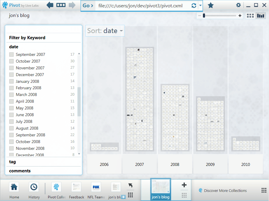
Pivot, from Microsoft Live Labs, is a data browser that visualizes data facets represented as Deep Zoom images and collections. I’ve been meaning to try my hand at creating a Pivot collection. My first experiment is a visualization of my blog which, in its current incarnation at WordPress.com, has about 600 entries. That’s a reasonable number of items for the simplest (and most common) kind of collection in which data and visuals are pre-computed and cached in the viewer. Here’s the default Pivot view of those entries.
The default view

To create this collection, I needed a visual representation of each blog entry. I didn’t think screenshots would be very useful, but the method worked out better than I expected. At the default zoom level there’s not much to see, but you can pick out entries that include pictures.
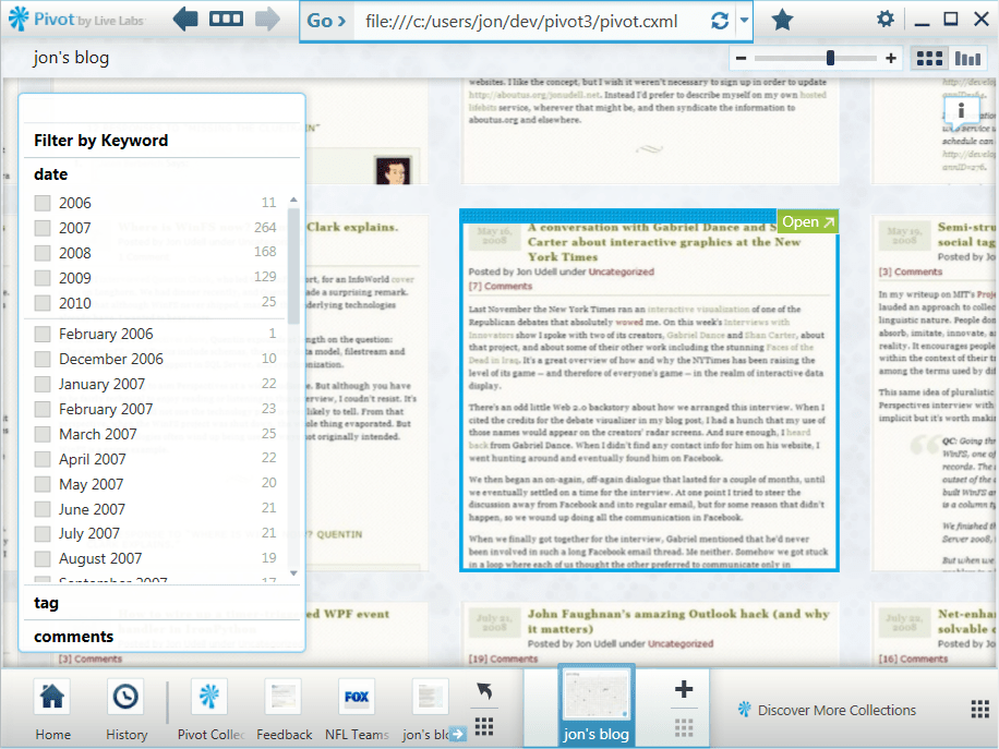
A selected entry
When you select an entry, the view zooms about halfway in to focus on it.
A text-only entry
Here’s a purely textual entry at the same resolution. If you click to enlarge that picture, you’ll see that at this level the titles of the current entry and its surrounding entries are legible.
The Show Info control
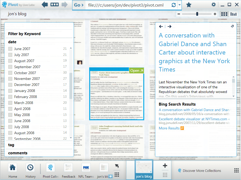
Clicking the Show Info control opens up an information window that displays title, description, and metadata. I’ve included the first paragraph of each entry as the description.
Zooming closer
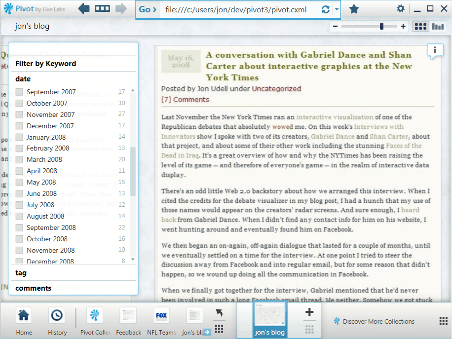
If I zoom in further, the text becomes fully legible.
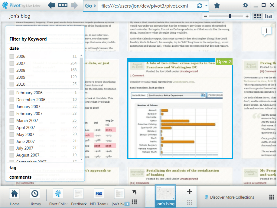
Histogram of entries
Of course the screenshot doesn’t capture the entire entry, it’s just a picture of the first screenful. To read the full entry, you click the Open control to view the entire HTML page inside Pivot.
Pivot itself isn’t a reader, it’s a data browser. This becomes clear when you switch from item view to graph view. 2006 and 2010 are incomplete years, but the period 2007-2009 shows a clear decline. I suspect a lot of blogs would show a similar trend, reflecting Twitter’s eclipse of the blogosophere.
2007 distribution
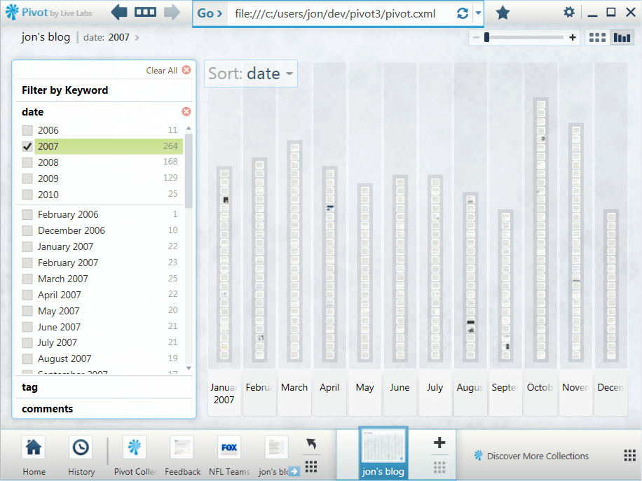
Here’s the distribution for just the year 2007.
Histogram of comments
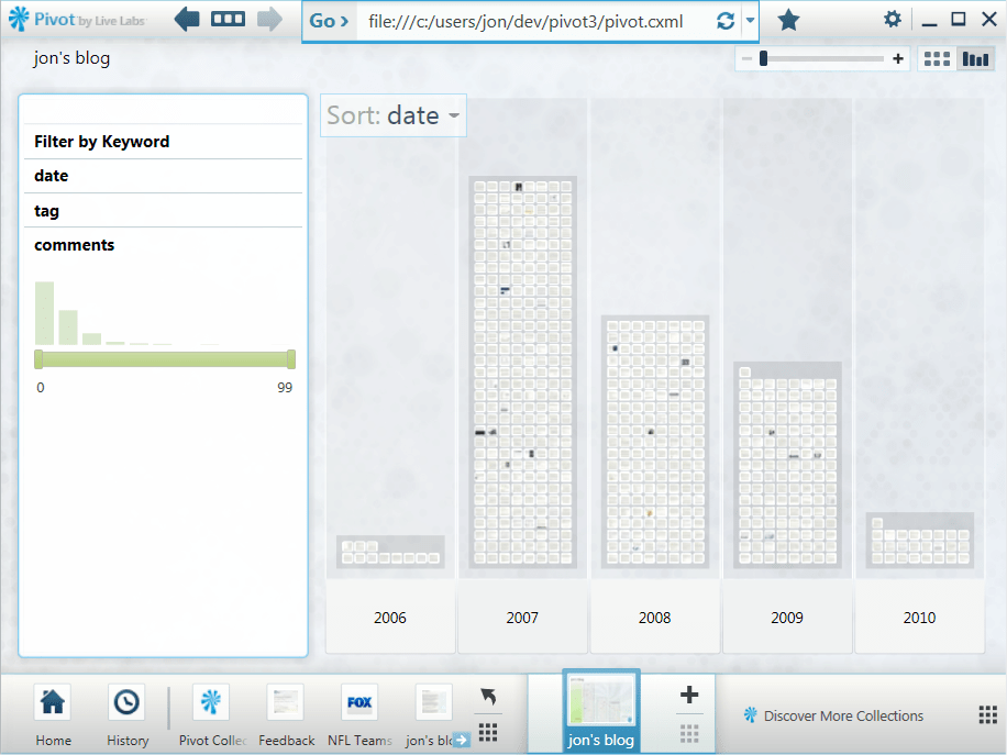
And here’s the comments facet, which counts the number of comments on each entry.
Histogram of entries with more than 20 comments
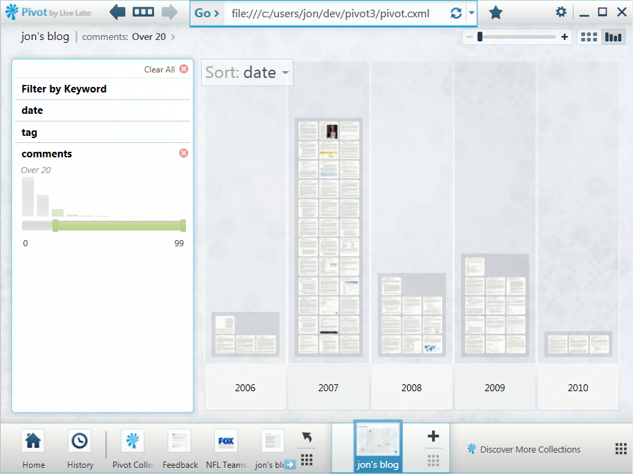
Adjusting the slider limits the view to entries with more than 20 comments.
Filtering by tags
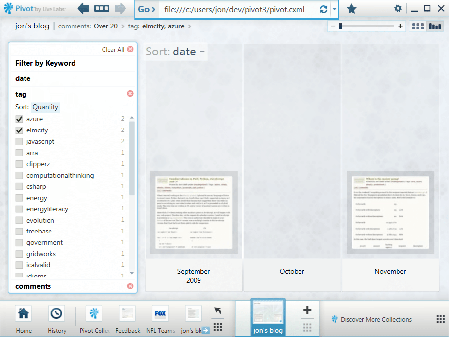
Of course I can also view entries by tags or tag combinations.
Filtering by keywords
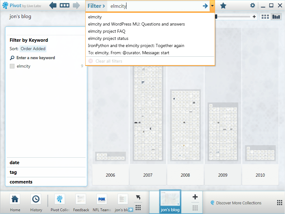
When I start typing a keyword, the wordwheel displays matches from two namespaces: tags and titles.
Other possible views
Facets can be anything you can enumerate and count. I could, for example, count the number of images, tables, and other kinds of HTML constructs in each entry. That isn’t just a gratuitous exercise. Some years back, I outfitted my blog with an XQuery service that could search for items that contained more than a few images or tables, and it was useful for finding items that I remembered that way.
It would also be nice to include facets based on the WordPress stats API. And since a lot of the flow to the blog nowadays comes through bit.ly-shorted URLs on Twitter, a facet based on those referrals would be handy.
How I did it
Life’s too short to make 600 screenshots by hand, so the process had to be automated. Also, I want to be able to update this collection as I add entries to the blog. So I’m using IECapt to programmatically render pages as images, and the indispensable ImageMagick to crop the images in a standard way.
To automate the creation of Deep Zoom images (and XML files), I’m using deepzoom.py. (Note that I had to make two small changes to that version. At line 224, I changed tile_size=254 to tile_size=256. And at line 291 I changed PIL.Image.open(source_path) to PIL.Image.open(source_path.name).)
To build the main CXML (collection XML) file, I export my WordPress blog and run a Python script against it. I hadn’t looked at that export file in a long time, and was surprised to find that currently it isn’t quite valid XML. The declaration of the Atom namespace is missing. My script does a search-and-replace to fix that before it parses the XML.
I haven’t uploaded the collection to a server yet, because there are a bazillion little files and I’m still tweaking. Once I’m happy with the results, though, I should be able to establish a baseline collection on a server and then easily extend it an entry at a time.
If there’s interest I’ll publish the script. It’ll be more compelling, I suspect, once Pivot becomes available as a Silverlight control. Currently you have to download and install the Windows version of Pivot to use this visualization. But imagine if WordPress.com could deliver something like this for all of its blogs as a zero-install, cross-platform, cross-browser feature. That would be handy.


